Our ideal for the execution of the second experiment was to have 60 participants of 40 years and older. There would be two labs where the experiment would be held in alternating rooms over 3 days. The rooms would be in a quite part of the school as we had quite a lot of disturbance during the first experiment.
The first setback was the location. It wasn’t possible to have two classrooms for three days at the same time. There weren’t any rooms available in a quiet part of the school. Eventually there was no other choice then to use a room in the middle of the busy documentation centre and spread the experiments out over 5 days. The room was a kind of aquarium, it was very light and you could see people walking around through the glass walls. During the test there was disturbance from talking and students opening the lab door by mistake. So far from ideal.
But my main disappoint was with the sample. Only one day before the start of the experiment the students notified me that they had managed to only get 20 participants instead of the 60 we had agreed upon. We were mostly depending on the teachers for participation but it was the period of the preliminaries and they were very busy. Also the trial would now take 40 minutes instead of the 20 to 30 minutes the first experiment took. Had I known earlier I could have taken steps and come up with a suitable solution.
As it was I had to improvise. I had to let go of the control group and had to broaden the age range. In the end 6 students of below 30 years old took part. I asked around in my own network and managed to recruit 10 people in the right age group. In the end we tested 40 people, all of whom were exposed to the stress stimulus.
Unfortunately not all the results were valid and useful. Some data was lost due to technical problems. Also quite a number of people made mistakes with filling in the questionnaires. We now had two questionnaires, one for self reported stress and one for self reported relaxation. The stress questionnaire contained one question in the positive direction (I feel everything is under control) and two negative items (I feel irritated, I feel tense and nervous). Both had to be reported on a 10 point scale.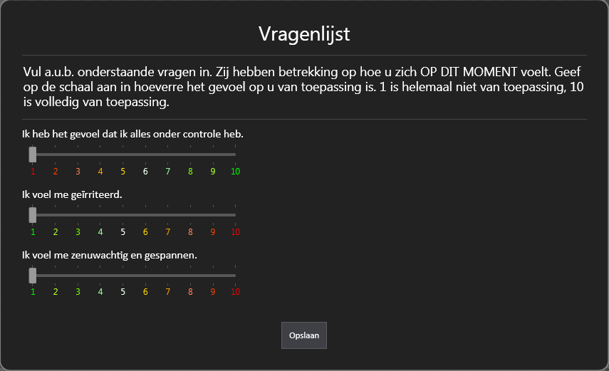 Apparently this was confusing for some people and even thought notes were taken it wasn’t always possible to reconstruct the correct answer. In the next experiment will put also some text below the numbers to indicate the value.
There were also two very extreme results (outliers), they can’t be included in the data set as they would mess up the averages too much. So I ended up will 33 data sets I could use for my analyses.
But first the data had to be sorted and structured. It took me quite some time to streamline the copious EventIDE output into a useful SPSS dataset.
The baseline measurement included self reported stress (pink), heart-rate (orange) and heart-coherence (red) and self reported relaxation (green). 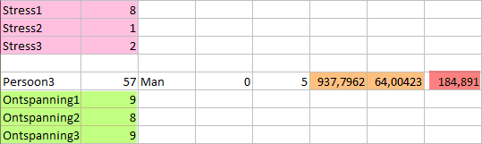
The three answers from all the questionnaires had to be combined into one value and checked for internal validity in SPSS.
It’s nice to take a look at a part of the results from the cognitive stress task:
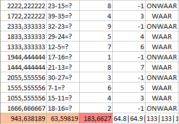
From the output you can see exactly what the sums were, how much time it took to make them, what the answer was and if the given answer was correct or not. I didn’t use this data but it would be nice to see if for example participants with more faults have higher heart-rates. Heart-rate (orange) and heart-coherence (red) are again below the results.
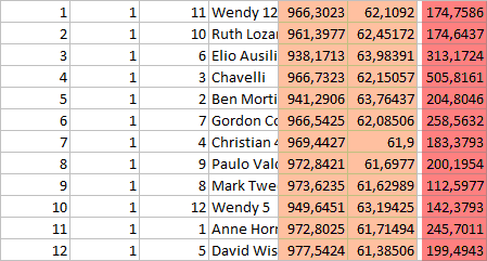
Before each stimulus set there was the stress questionnaire and after each set the relaxation questionnaire. The output for each set, which consisted of 12 pictures with sound is laid out as follows:
Picture count | set number | image id | image name | inter beat interval | BPM | heart-coherence
Each picture was shown for 20 seconds and the heart data was logged around four times per second. The output for one picture looks like this: 60.6|60.5|60.4|60.9|61.2|61.5|61.7|61.8|61.9|61.9|61.9|61.9|61.9|61.9|61.8|62.6|63.1|63.5|63.7|63.5|63.3|63.2|63.2|63.1|63.7|63.8|63.9|63.4|63.1|62.9|62.7|63.1|63.5|63.6|63.6|63.7|63.7|63.8|63.8|63.8|63.4|63.2|62.9|62.8|62.9|62.9|62.9|62.9|62.6|62.2|62.1|61.8|61.5|61.3|61.2|61.1|61.1|61.0|60.9|60.8|61.1|61.3|61.4|61.5|61.6|61.6|61.7|61.7|61.7|61.5|61.3|61.3|61.2|61.2|61.0|60.9|60.8|61.0|61.1|61.2|61.2|61.2|61.3|61.3|61.4|61.4|61.0|
This yields an average of 62.1 which is the output I used. But it is good to have all this data for each individual image. All the image averages had to be combined in a set average so I could easily analyse the differences between all three sets. I’m still analysing the data. More on that in my next post.